Sometimes it is useful to show variation, events, etc. over time and space, perhaps for a departmental talk or conference presentation. A common way to do this is with a static map where the coloring of the dots correspond to time. Let’s say we want to show when and where colleges and universities opened in the U.S. This might look something like:

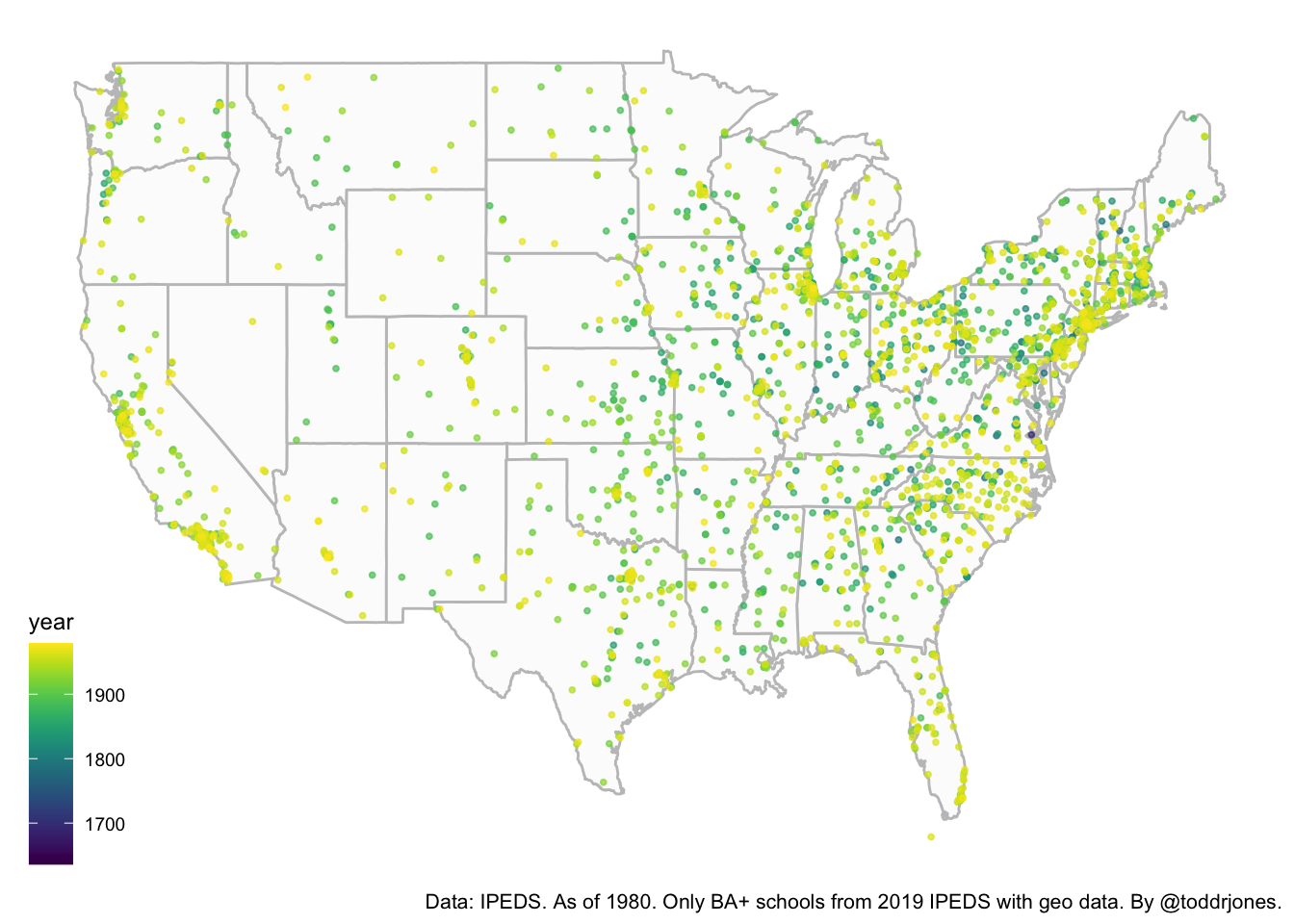
This is OK, but because there are so many, some of the earlier schools get covered over by the later. It is also jumbled and can be hard to see what is going on.

Another way to do this, and this focus of this post, is to create an animated map. In some cases, this is easier for the audience to quickly understand. What follows is an example of how to do this using R code.

First load the necessary packages:

library(tidyverse)
library(ggplot2)
library(dplyr)
library(gganimate)
library(ggthemes)

Set your working directory as applicable.

setwd("/")

We will use two data files from IPEDS at this link. First is the Institutional Characteristics file from 1980 (I am using this year because it has the year the university started.) Select “1980” and “Institutional Characteristics” and download the “IC 1980” data file.

The second is the 2019 Institutional Characteristics file (this has latitude and longitude; analysis will be limited to institutions in this file). Download this from the above link by selecting “2019” and “Institutional Characteristics.” We want the “HD 2019” data file. You can also download them here. In what follows, the files are saved in the “files” folder.

Load the data, merge, clean, and make a few sample restrictions:

#read in data
data1980 <- read.csv("files/ic1980.csv")
data2019 <- read.csv("files/hd2019.csv")

#rename variable
names(data2019)[1] <- "unitid"

#merge the two files together
data <- merge(data1980, data2019, by="unitid")

#keep only BS and higher institutions
data <- data %>% mutate(var1=ifelse(INSTCAT==1|INSTCAT==2, 1, 0))

#keep only public and private (exclude for profit)
#in original version, there are 28 for profits
data <- data %>% filter(control!=0)

#keep selected columns
data <- data[,c("INSTNM", "unitid", "estmoyr",
                "LONGITUD", "LATITUDE", "control")]

#change a couple variable names
names(data)[4] <- "longitude"
names(data)[5] <- "latitude"

#drop the ones missing year
data <- data %>% drop_na(estmoyr)

#extract last four digits, which is year
data$year <- sub('.*(\\d{4}).*', '\\1', data$estmoyr)

#sort by year (just to be able to better see the data)
data <- data %>% arrange(year)

#get rid of observations outside of map area
data <- filter(data, data$longitude>-125.5)
data <- filter(data, data$longitude< -66)
data <- filter(data, data$latitude >23.5 & data$latitude < 49.5)

#change the data type of a couple of variables
data$year <- as.integer(data$year)
data$control <- as.factor(data$control)

We can then animate the plot. The gganimate package will do the heavy lifting. The transition_time, shadow_mark, and labs code are all related to gganimate. The way it works is that it shows the college openings for each year separately (governed by transition_time). It then keeps the dot there (with shadow_mark). The label comes from labs, where frame_time is the year.

map <- ggplot(data, aes(x = longitude, y = latitude, group=unitid)) +
    borders("state", colour = "gray76", fill = "gray97") +
    theme_map() +
    geom_point(alpha = .5, colour = "black", size=1, show.legend = FALSE)   +
    labs(caption = "Data: IPEDS. As of 1980. Only BA+ schools from 2019 IPEDS with geo data. By @toddrjones.")+
    theme(plot.title = element_text(hjust = 0.5)) +
    theme(plot.subtitle = element_text(size=16, hjust = 0.5, vjust=-4)) +
    transition_time(year) + 
    labs(subtitle = paste('Year: {frame_time}')) +  
    shadow_mark(colour = '#0072CE', size=4, alpha=.6) +
    theme(plot.title = element_text(size=16)) +
    theme(plot.caption = element_text(size=8))
    
#Note that you can save as a .gif file by doing something along the lines of:
#anim_save("colleges.gif", map, end_pause=15, width = 600, 
#     height = 400, duration=17, nframes=400)

map